


The infinite coastline paradox
How unexpected difficulties in a practical measurement problem challenged fundamental conceptions of length and led to a new theory of dimension, while revealing monsters lurking at small scales.

A century ago Lewis Fry Richardson (1881–1953), noted polymath with prizes now named in his honor in metereology and scientific peace research, had a mathematical theory for predicting the likelihood of war between two countries based in part on the length and nature of their common border.
Aiming to test his theory, he looked into the details of various borders in Europe but found some strange disagreements—the Portuguese reported their border with Spain to be 1214 km, while the Spaniards thought it was 987 km long; the border between the Netherlands and Belgium was reported as 380 km or 449 km; and similar disagreements held for many other borders. Curiously, when two countries shared a common border, it was typically the smaller country reporting a larger value. Why should there be such a level of disagreement about such basic measurements, especially one of vital importance for issues of sovereignty?
Richardson pondered the manner in which one calculates the length of a border or coastline. Naturally, one lays off unit segments on a large, detailed map—perhaps the map is 50 kilometers to the centimeter and one lays these off as unit segments, counting their number to find our estimate. Using smaller unit segments would presumably give a more accurate result, right?
What Richardson found, however, was that smaller units often led to a huge increase in the estimated length. And using a still smaller unit segment would make another unexpected increase. The total estimated length of the border did not seem always to stabilize but in practice was sensitive to the scale of measurement. Richardson began to realize a basic incoherence of the concept of a determinate length for a given border, and introduced an invariant for calculating how the estimated length would scale larger as the unit of measurement became smaller—a deeply insightful contribution anticipating later developments of Benoit Mandelbrot. Even infinite border lengths remained a theoretical possibility.
Measuring the length of a coastline
How long is the coastline of Great Britain? Consider the measurements indicated in the animated figure here.
On the coarse end of the scale, we use a comparatively crude unit measurement scale of 150 km, finding the estimated coastline length to be 2610 km. In the middle of the animation, with a considerably finer measurement unit of 4.4 km, we resolve many more of the bays and river inlets, more than doubling the measured coastline length to 6220 km. At the finest end of the scale, with a measurement unit of 50 m, we find far more detail, nearly doubling the length estimate again to 11500 km.
The accompanying graphs show how the length estimate varies with the measurement unit, generally producing longer estimates with smaller scales. Since this is a logarithmic scale, the basically linear appearance of the graph indicates an exponential growth relationship between the length estimates and the measurement scale. The slope of that line is essentially the invariant that Richardson had found—different coasts and borders will each exhibit their own characteristic slope, depending on the topographical and geographic nature of that border.
Notice particularly the zoomed-in region of the coast in the Scottish Highlands—it is the coastal region from Loch Alsh to Loch Hourn—which clearly shows the phenomenon in play. The crude measurement unit of necessity passed completely over the details of this region, while the medium-fine scale was able to follow some of the ins and outs of the coastline. The finest measure resolved a considerably longer coast, precisely because it was able to follow the river inlets and bays much further. This is precisely the process by which a finer measure leads inevitably to a longer coastal estimate.
Benoit Mandelbrot (1967), building on Richardson's ideas, mounted the theory of fractals to explore the strange new theory of this entirely new class of curves and geometrical objects, introducing the fractal dimension, building on the Richardson invariant anticipated earlier.
The subject of fractals thus finds its origin in a practical problem—measuring the length of a border or coastline—but gives rise to a new mathematical theory, one concerned with the purely mathematical features of the abstract mathematical objects of our imagination. The puzzling theoretical examples shed light on our core conceptions of the nature of the length of a mathematical curve and even our conceptions of dimensionality.
Paradoxes of perimeter
Let us adopt this coastline measurement way of thinking to consider few natural attempts to approximate the values of √2 and π.
Length of a diagonal
Consider the diagonal of a unit square, as shown in the figure here.
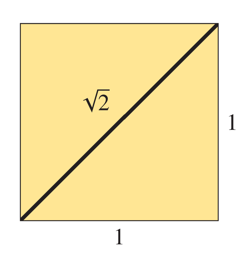
The sides have unit length 1, and so the diagonal has length √2 by the Pythagorean theorem. Let us try to calculate approximations to √2 by constructing increasingly fine approximations to the diagonal using simple finite combinations of linear segments in such a way that we can easily calculate their total length.
Consider, for example, the series of increasingly tight staircases illustrated in the figure below. As the number of steps becomes very large, it will become difficult to distinguish the staircase approximation from the diagonal itself.
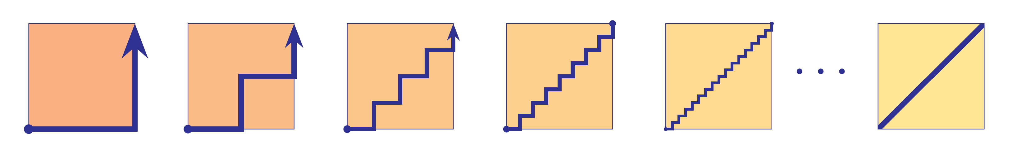
How well did we do? Let's calculate the lengths of the approximations and observe how well they approximate √2 as the resolution becomes very fine. The very first staircase at left, following the bottom edge and then the right-side edge of the square, has total length 1+1 = 2. Crude, but perhaps an acceptable start. The second staircase has four segments, each of length 1/2, which makes again a total length of 2. Hmmnn…it didn't change. The third staircase approximation has eight segments of length 1/4, again making a total length of 2. Wait, what? Why isn't it converging to √2? The next approximation has sixteen segments of length 1/8, again with total length 2. Indeed, we may observe that all the staircase approximations, no matter how fine the resolution, will have a total length of 2, because for each staircase the sum of all the horizontal segments will be 1 and the sum of the vertical segments will be 1, making the total length 2. The strategy of approximating √2 this way is a total failure! What is going on? Although the staircases seemed to approximate the diagonal to an increasing fine degree, they all have length 2, whereas the diagonal has length √2, and we know these are not the same. How can one explain this paradox?
Circumference of a circle
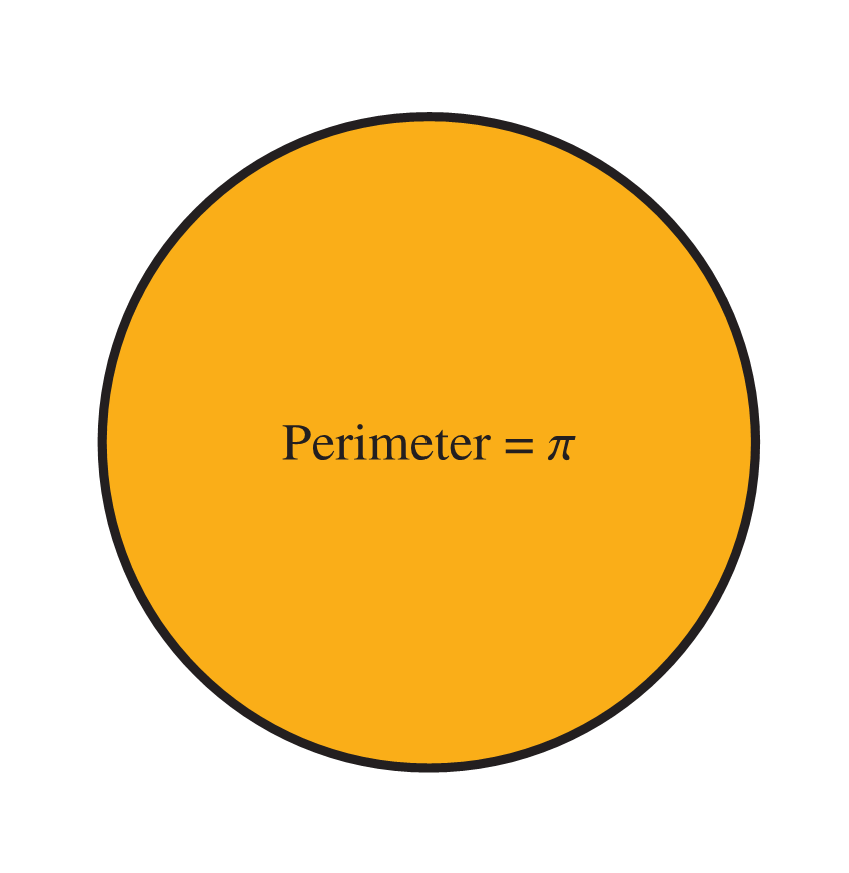
Here is another similar instance—we shall try to calculate an approximation to π. Start with a circle of diameter 1, which consequently has a circumference of exactly π.
We place the circle in a square box, as shown below at left, and proceed successively to remove corners from the box so as to make the boundary of the enclosing box more and more closely approximate the circle. Keep trimming the corners to make the bounding box as close to the circle as you can. Eventually, with a very fine resolution, the bounding box will become indistinguishable from the circle.
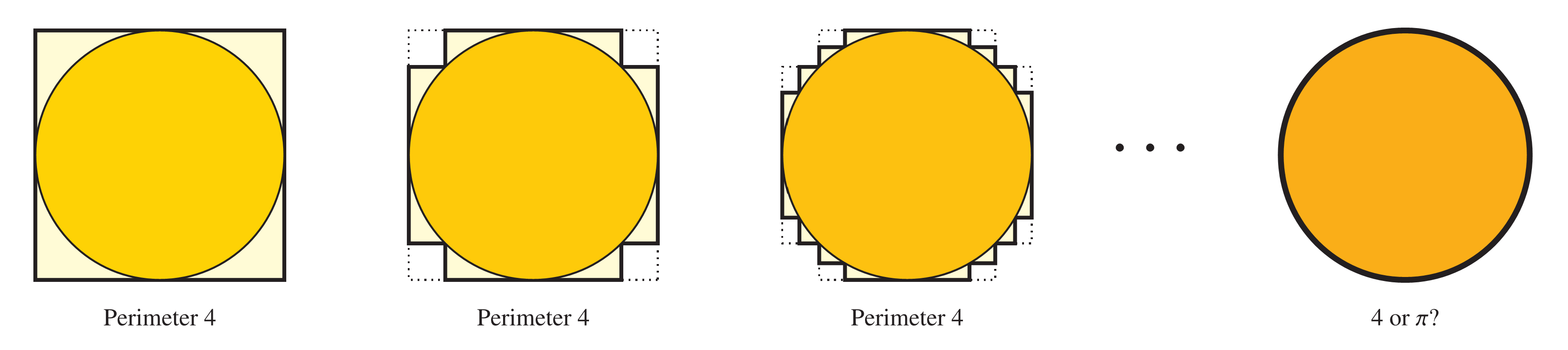
How well do the approximations approximate π? The initial square has four sides of unit length, which makes a perimeter of 4. A crude estimate, to be sure, but perhaps acceptable as a first approximation. For the next box, let's consider how long is the perimeter. How shall we calculate it? Do we need to know further details about exactly which points were used when pushing in the corners? No, we don't, because the process of removing a corner from a box actually preserves the perimeter, since it simply replaces a vertical/horizontal arrangement with a horizontal/vertical arrangement of exactly the same length. And so the second box actually also has perimeter 4. But wait, hmmmnn. The very same argument shows that the third box also will have perimeter 4, and indeed all the bounding boxes will have the same perimeter of 4, since the process of pushing in a corner does not change the perimeter. Unfortunately, this method of approximating π has also been a total failure. We know that π is definitely less than 4, simply by considering the very first box. What is going on?
The length of a curve
The problem with the previous paradoxical examples is that they rely on a subtly faulty notion of what it means to have an approximation to a curve. With the right conception, we shall realize that we were mistaken about the staircases and bounding boxes—we should not regard them as approximating the curves in a way that is useful for estimating the length.
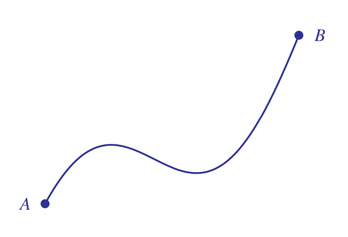
So what does it mean to have an approximation to a curve or to speak of the length of a curve? To be sure, we know how to conceptualize and measure the length of a straight line segment. We can use the distance formula, for example, which is really just another way of thinking about the Pythagorean theorem. But when a curve is really curvy, what does it actually mean to refer to the length? Consider the elegant curve here, climbing gracefully from point A to B. What does it mean to speak of the length of this curve?
We can provide a robust conception of the length of a curve by considering its piecewise linear approximations—we select any finitely many points on the curve and join them with linear segments.
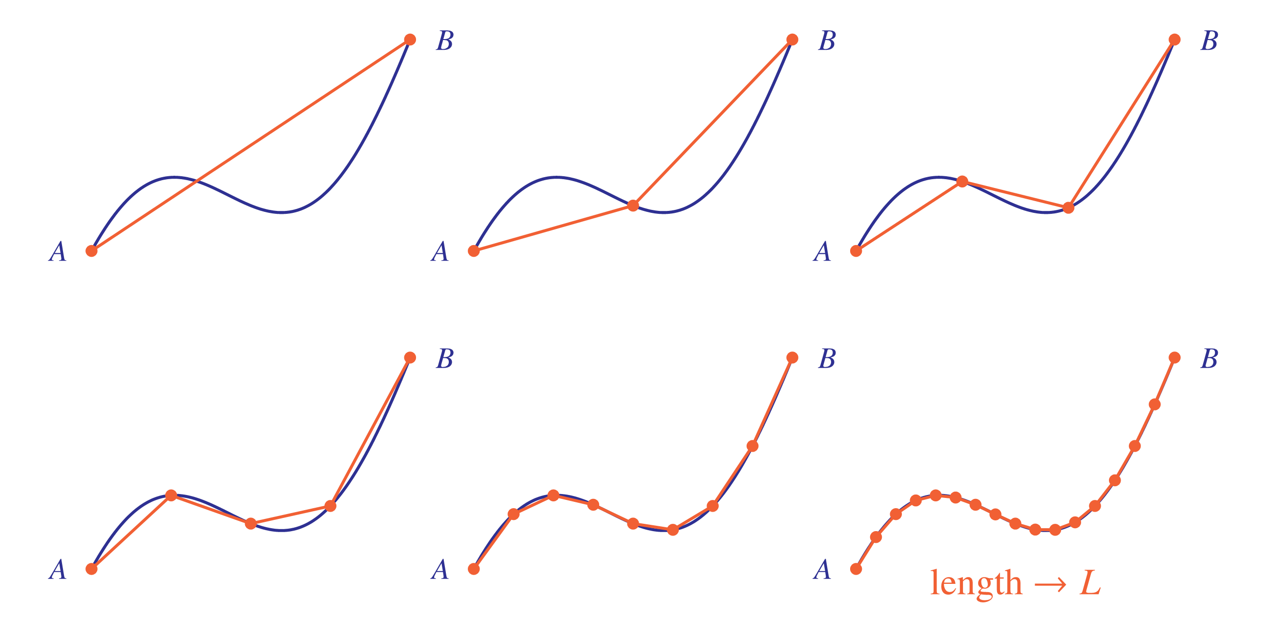
As we take more and more points, these linear approximations may converge to a limit value L, and in this case we say that the length of the curve is L. Since the curve is at least as long as any piecewise linear approximation, we can simply define the length of the curve to be the supremum of the lengths of its piecewise linear approximations. A curve is rectifiable when this limit exists—in this case, the curve is well approximated by linear segments and it has a well-defined length.
OK, what is the difference between this rectifiability idea and the approximations we had considered earlier? The difference is that in order to fulfill rectifiability, we consider linear approximations consisting of segments joining points on the curve. But the staircase and bounding box approximations, in contrast, were criss-crossing the curve, often making turns at points not on the curve. These inefficient excursions away from the curve caused wasteful extra length in the approximations, making them systematically too long, and this is why we don't want to count them as piecewise linear approximations. Indeed, those deviations from piecewise linearity explain why those approximations each had a longer length than expected, thereby resolving the paradoxes.
Archimedes approximates π
Mathematicians often regard the concept of rectifiability and the limit process I described above as part of the core collection of ideas underlying the differential calculus. And yet, nearly two millenia before Newton and Leibniz and the calculus, Archimedes famously used the method of piecewise linear approximation to calculate some prescient early approximations to π. Perhaps this shows how close Archimedes was to discovering the calculus.
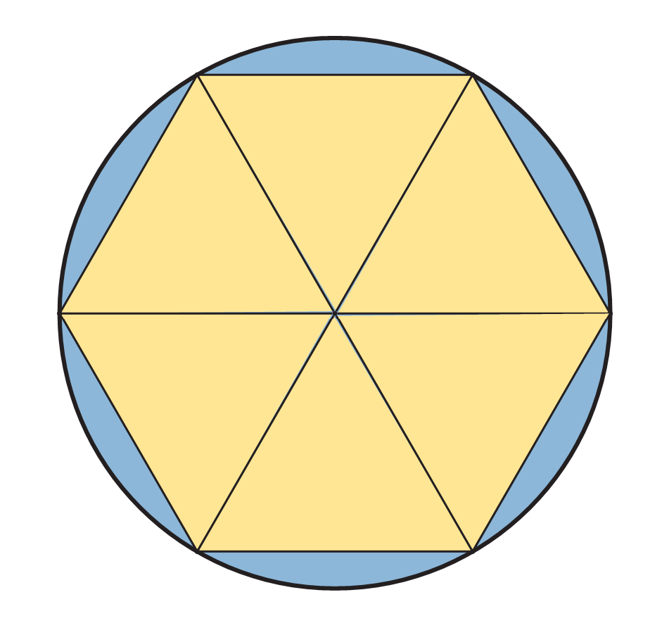
Consider the unit circle shown here, with radius 1. We inscribe a regular hexagon within it, consisting of six equilateral triangles, and so each side of the hexagon is the same as the radius of the circle. Thus, the perimeter of the inscribed hexagon is exactly 6, while the perimeter of the circle is 2π. Since the straight sides of the hexagon are shorter than the curved segments of the circle—they form a piecewise linear approximation of the circle in the sense of rectifiability—it follows that 6 < 2π, and therefore:
This is our first approximation of π.
Archimedes established better bounds on π by extending the inscribed hexagon to an inscribed 12-gon, and then subsequently an inscribed 24-gon, and so on. Let us consider how one might argue with just the regular 12-gon, shown here, formed by bisecting the equilateral triangles of the inscribed hexagon each with a radius of the circle, making twelve angles of 30° at the center.
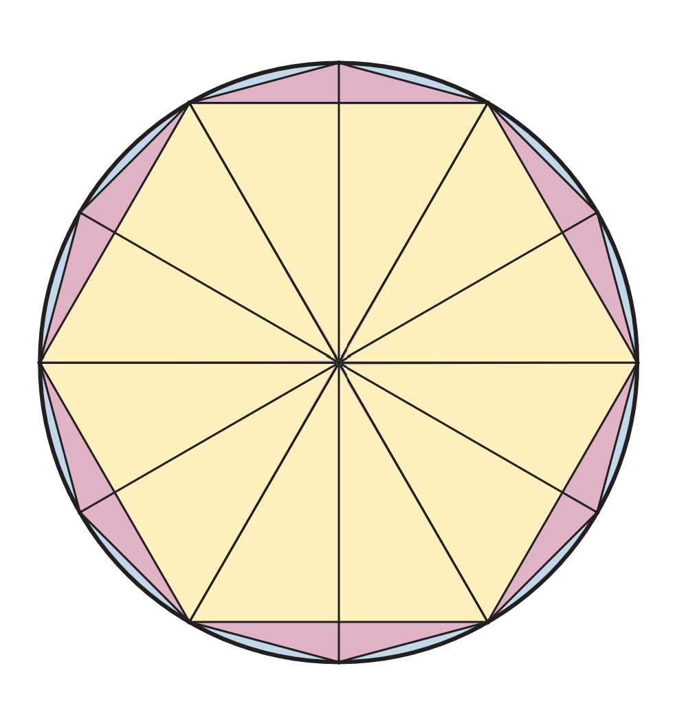
If you consider the twelve small purple triangles that are added around the circle as a result, the leg bordering on the hexagon has length 1/2, since it is half of the original equilateral-triangle side; the other very small leg on the radius has length 1 - √3 / 2, since it is what remains of the radius 1 after the equilateral-triangle altitude of √3 / 2. So by the Pythagorean theorem, the perimeter segment of the 12-gon, which is the hypotenuse of the small extra dark triangle, has length
which some simple algebraic manipulation shows is equal to
Since there are twelve sides and the perimeter of the circle is 2 π, we may conclude that
One may calculate the value of the square-root expression as 3.1058…, and so in particular, this shows 3.1 < π.
The inscribed 24-gon has a perimeter of approximately 3.132, it turns out, and the inscribed 48-gon has a perimeter of approximately 3.139, and one thereby begins to see how to obtain increasingly better approximations to π this way. Using a regular 96-gon, Archimedes ultimately established that 223⁄71 < π < 22⁄7, which in decimal notation establishes
What can go wrong—nonrectifiable curves
Let us consider again the elegant curve that we had considered earlier, climbing gracefully from point A to point B.

Is it rectifiable? Does this curve have a well-defined length? It certainly seems to have a definite length, and earlier we had drawn a series of piecewise linear approximations, which seemed to be converging nicely. If indeed those approximations do converge, then this would be a rectifiable curve with a well-defined length. We seem to have a gentle, innocent, well behaved curve.
In order to be more certain, however, perhaps we should inspect the curve a little more closely. Shall we look at it under a microscope to see that there is nothing untoward?
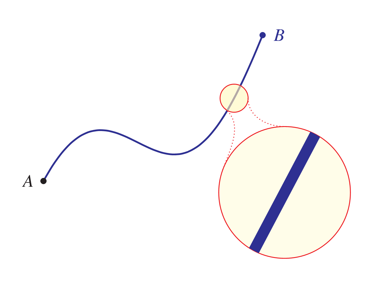
Here I have zoomed in on a particular part of the curve. Does it look acceptable? Does it still seem rectifiable? Yes, indeed, everything seems to be in order—the curve seems completely fine and well behaved. What could go wrong?
Our friend, who as a child was anxious about monsters hiding under the bed, insists we look closer. After all, he says, didn't you notice above that under the microscope the curve seemed weirdly thicker than we might have expected? What could be causing that? Our friend has a more powerful microscope (he carries it everywhere), and with it we can zoom in a bit deeper on that part of the curve. What does it reveal?
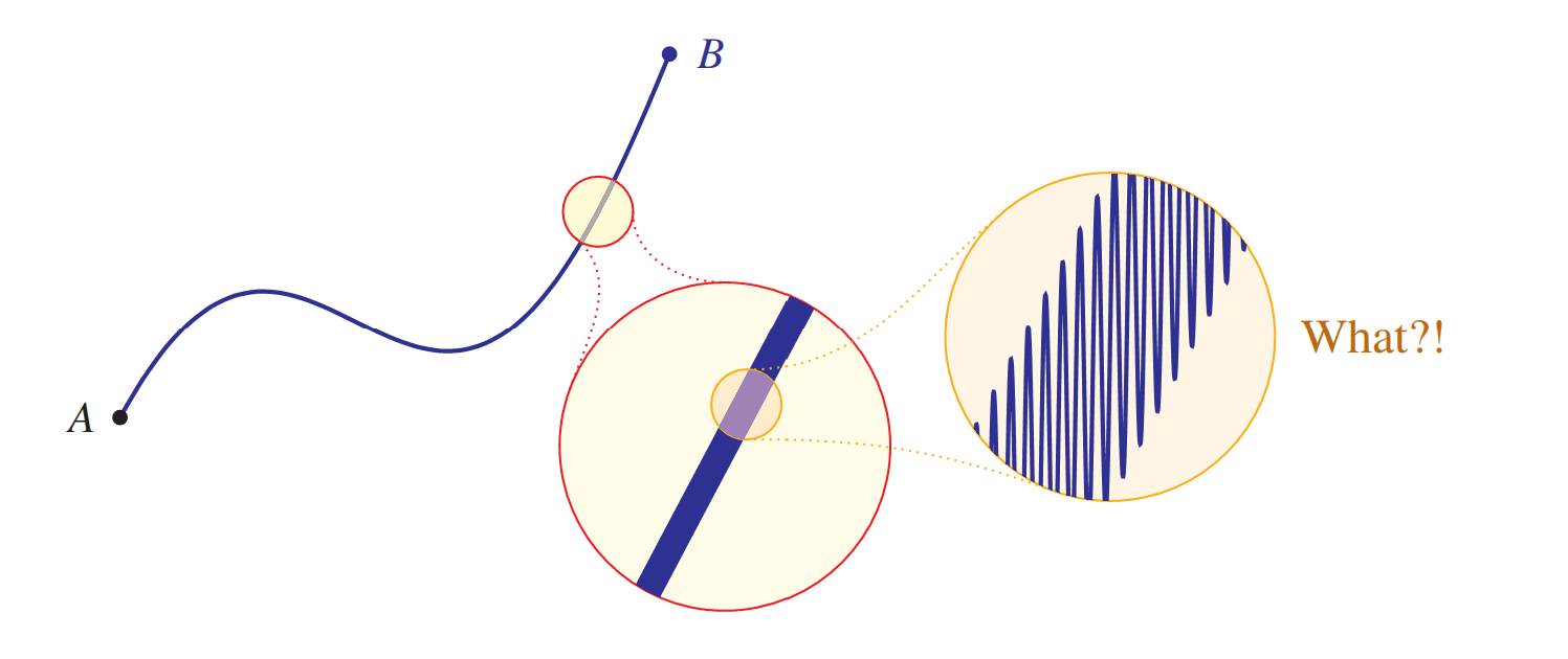
OMG! What is that?! Oh dear, we were completely mistaken in our judgement of the nature of the curve. What we had thought to have been a gentle upward-sloping rise in the curve was actually a chaotic scramble of violent upward and downward jerks. This explains why the curve seemed a little thicker than expected—it was indeed a monster in the small scale.
Notice the drastic effects of the violent up-and-down motion on the length of the curve. What we had thought to be an extremely short segment of curve, if we were measuring with a piece-wise linear approximation at the previous scale, is actually considerably longer by a large multiple. Each short segment of the original curve with this behavior is at least dozens of times longer than expected because of all the up and down motion. Although the absolute magnitude of those up-down jerks are miniscule, they cause a multiplicative factor in the length because of their number and density. Indeed, if the up-down zig zags were more tightly packed in, the actual length of the curve could have been much longer than expected by an enormous factor, perhaps millions of times as long as expected.
Suppose we zoom in even closer? We might look closely at one of those violent zig zags. Perhaps at a tighter scale, it will look fine, like the narrow parabola shown on the green background here.
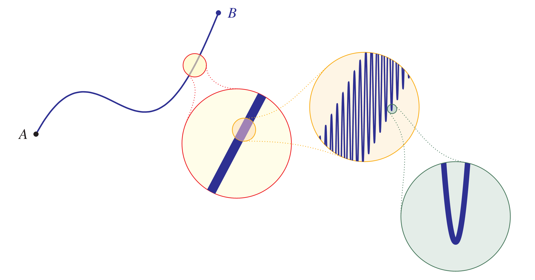
Whew! Everything seems good. But wait, our anxious friend insists that we look still closer again.
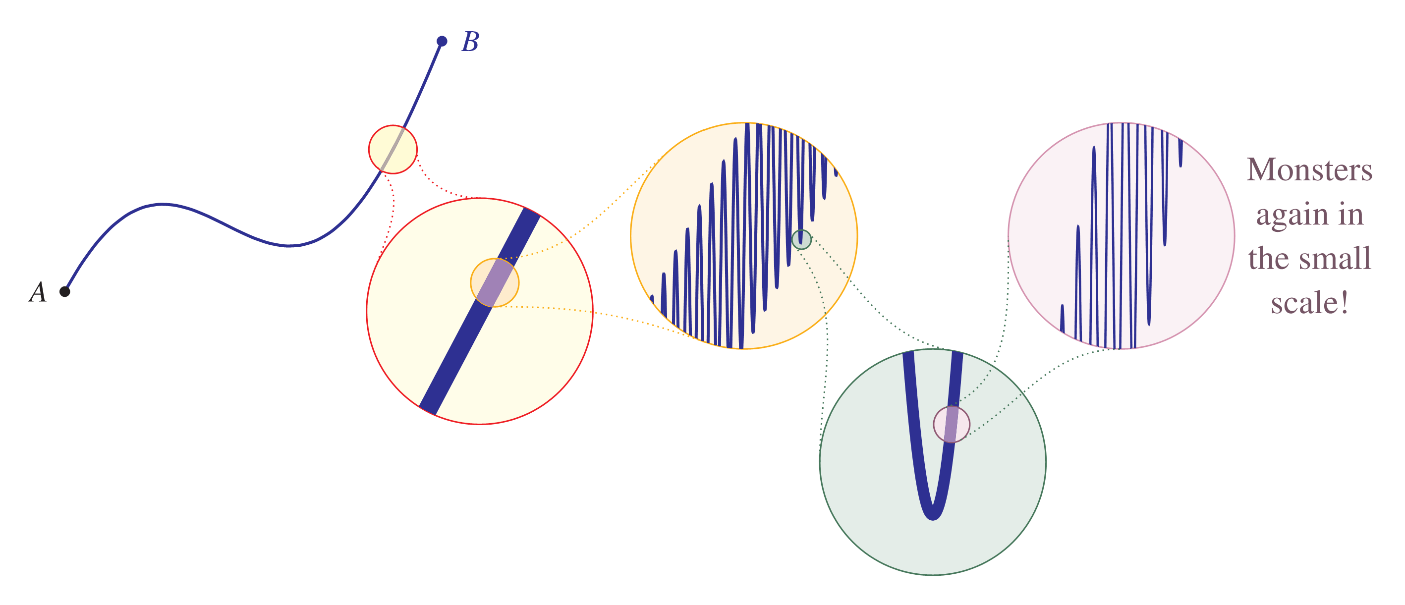
Oh no! We've found a deeper tinier realm of violent action, occurring at a much smaller scale of resolution. The curve overall appears nice and smooth at some scales, yet chaotic and scrappy at other scales.
The main point I want to make is that essentially any curve we observe might exhibit this kind of monstrous behavior at small scale. Are we surrounded by mathematical monsters? Perhaps all the functions we've been plotting and graphing and analyzing are like this, when we zoom in close enough. And if it occurs often enough or badly enough, then the curve will not have a rectifiable length. The increasing multiplicative factors could cause the total length of the curve from A to B to become infinite.
Let me point out briefly, for those readers who are familiar with the calculus concept of the derivative, that because of the monstrous behavior at very small scale the elegant function we considered from A to B has a truly monstrous derivative and not just at small scales. Although initially the slope of the curve looked quite tame, perhaps with a slope everywhere bounded by about 2, nevertheless the small-scale violent behavior we observed causes the actual slopes to be MUCH higher—the chaotic up and down motion is extremely steep where it occurs, making the values of the derivative swing from enormous positive values to enormous negative values and back again. The derivative of this function is not nice.
Fractals
The class of curves known as fractals often illustrate this kind of behavior in a systematic self-reflective manner. Let us explore a few examples.
Koch snowflake
Consider the Koch snowflake curve, which despite its complexity is generated as the limit of a sequence of approximations according to a surprisingly simple underlying rule.
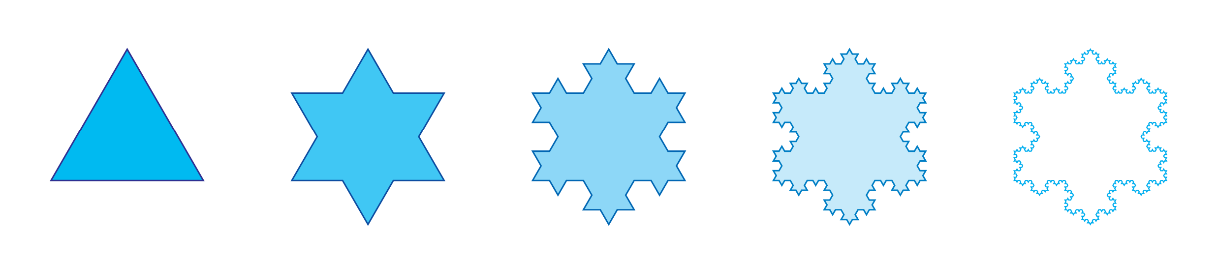
Namely, the first approximation to the Koch snowflake curve is an equilateral triangle, at left; and at each stage of approximation, the generation rule for the next stage is simply to replace each of the straight line segments, at whatever scale they appear in the current approximation, with a corresponding four-segment notched version as shown below. Thus, each little segment gets a notch in it, and then the notches get tinier notches and so on ad infinitum.

Can you see how this rule transforms each snowflake approximation into the next? At each stage of generation, these approximations will be piecewise linear approximations to the final snowflake curve, which is the limit of these approximations.
The important thing to notice about the curve-generation process from the perspective of rectifiability is that the notched replacement configuration consists of four segments, each one third of the length of the original segment. The length of the replacement is therefore 4/3 times as long as the original segment. Perhaps it helps to realize that the original segment consists in effect of three one-third segments, but afterwards we have four one-third segments, which is therefore one-third longer, a factor of 4/3. Precisely because every segment is replaced in this way, it means that at every stage of approximation, the total length of the approximation grows by a factor of 4/3.
Sierpinski gasket
The Sierpinski gasket, another fractal shown here, is also generated by a simple replacement rule.
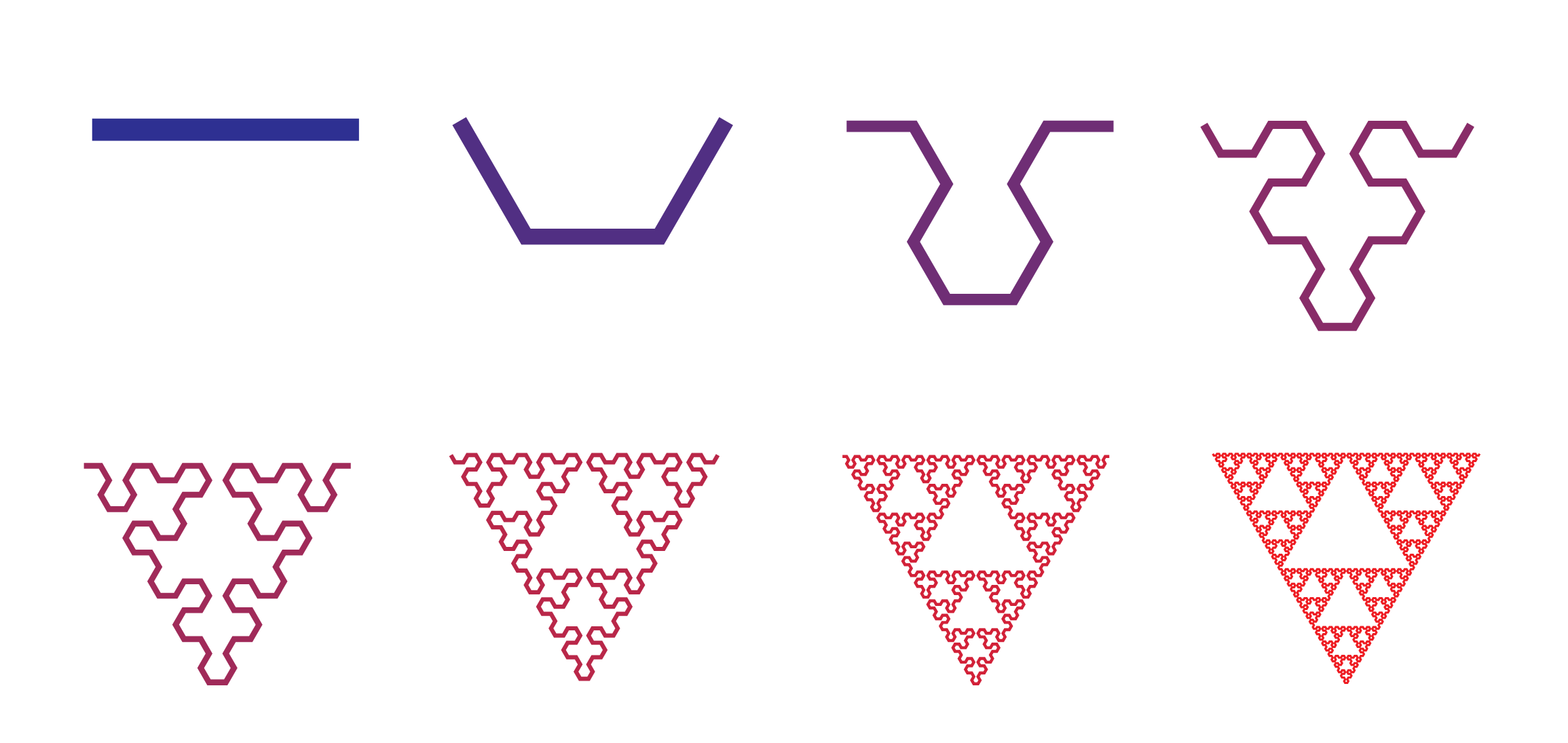
The unit operation replaces each segment with the three-segment arrangement, alternating the orientation. These images were generated by an algorithmic process that literally performed that process iteratively.
The resulting limit curve has infinite length.
Fractal dimension
The fractal curves we just considered open the door to a fascinating observation about fractional dimension. Some curves are best described as having a particular numerical dimension strictly between 1 and 2. What does it mean?
Consider first how scaling works in various familiar dimensions. If we scale a linear segment by a linear factor of two, it becomes twice as long—we get two copies of the segment. If we scale a square up by a linear factor of two, however, meaning that each side becomes twice as long, then we get a square with four times the area, four copies of the original. And scaling a cube by a linear factor of two gets us eight copies of the original cube. In general, in dimension d, scaling by a linear factor of s results in an object that is sd times as large in the d-dimensional sense.
This formula works when scaling downward also, when s < 1. Scaling a square (down) by a factor of s = 1/3, that is, making the side lengths one third the size, makes the area s2 = 1/9 as large—we have divided the square into a 3 × 3 array of nine smaller squares, each one third the linear size.
How does this dimensional analysis apply to fractals such as the Koch snowflake and the Sierpinski gasket? If you inspect the final Sierpinski gasket shape, you will see that it exhibits a self-similarity by which the entirety of the figure consists of three copies of itself, each scaled down by a linear factor of two. In other words, doubling the linear scale caused an increase in size of 3. But what dimension is like that? It must be somewhere between 1 and 2, since for those dimensions we would get an increase in size of 2 or 4, respectively. We can find out the exact dimension of the Sierpinski gasket by solving the equation 3 = 2d. Taking logarithms of both sides, we see that log 3 = log 2d = d log 2, and so d = log 3 / log 2, which is about 1.5849. Thus, the dimension of the Sierpinski gasket is between 1 and 2, slightly closer to 2. Perhaps this fits with appearances, since in a sense the gasket begins almost to fill out a two dimensional area in the plane but not quite fully.
For the Koch snowflake curve, notice how each component exhibits a self-similarity by which it consists of four copies of itself, each scaled down by a linear factor of 1/3.
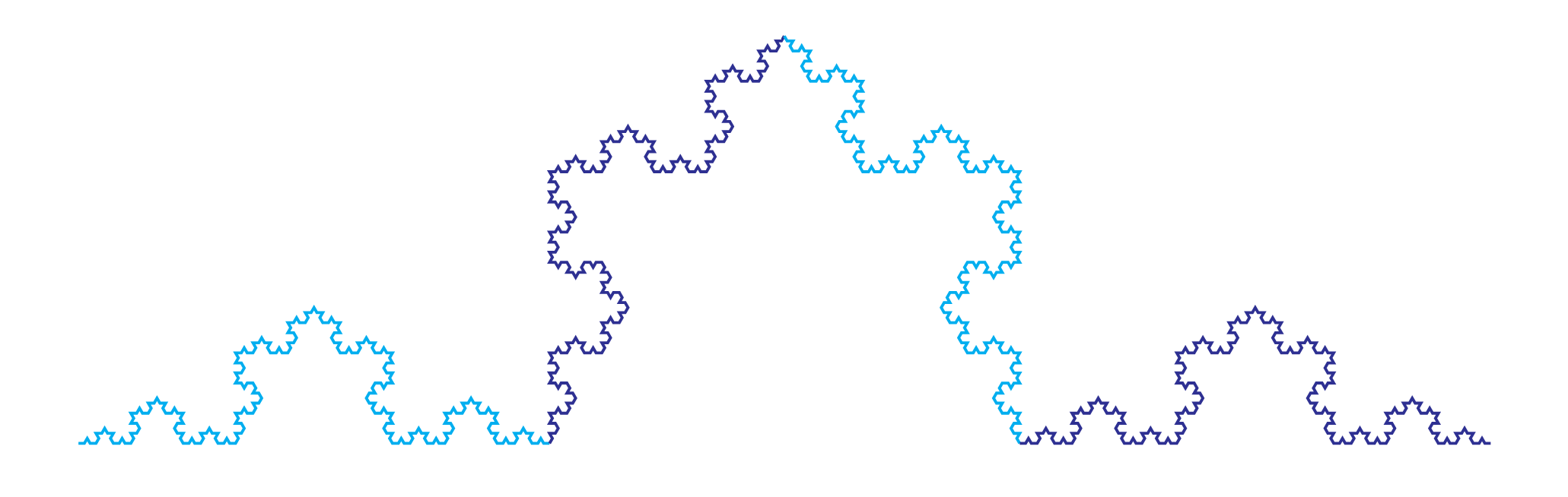
Thus, tripling the linear scale caused an increase overall of four. This corresponds to a fractal dimension of d solving the equation 4 = 3d, which again by taking logarithms has the solution d = log 4 / log 3, which is about 1.262. So the snowflake curve also has a dimension strictly between 1 and 2, but closer to 1 than 2, and less than the Sierpinski gasket, which perhaps fits with appearances, since the snowflake curve seems much less two-dimensional than the Seirpinski gasket. And yet, it is more than merely one dimensional.
Space-filling curves
What other monsters might there be in the small scale? How strange and unwieldy can a curve be? Very strange, indeed. Consider the phenomenon of space-filling curves, curves that entirely fill a solid region of the plane or space in which they reside. Giuseppe Peano was the first to provide such curve, but let us explore David Hilbert's simplified variation.
Like the fractals we saw earlier, the Hilbert curve is defined by a limit process. One starts with the crude approximation below at left, consisting of three line segments, and then each approximation is successively replaced by one with finer detail, and the final Hilbert curve itself is the limit of these approximations as they get finer and finer. The first six iterations of the process are shown here.
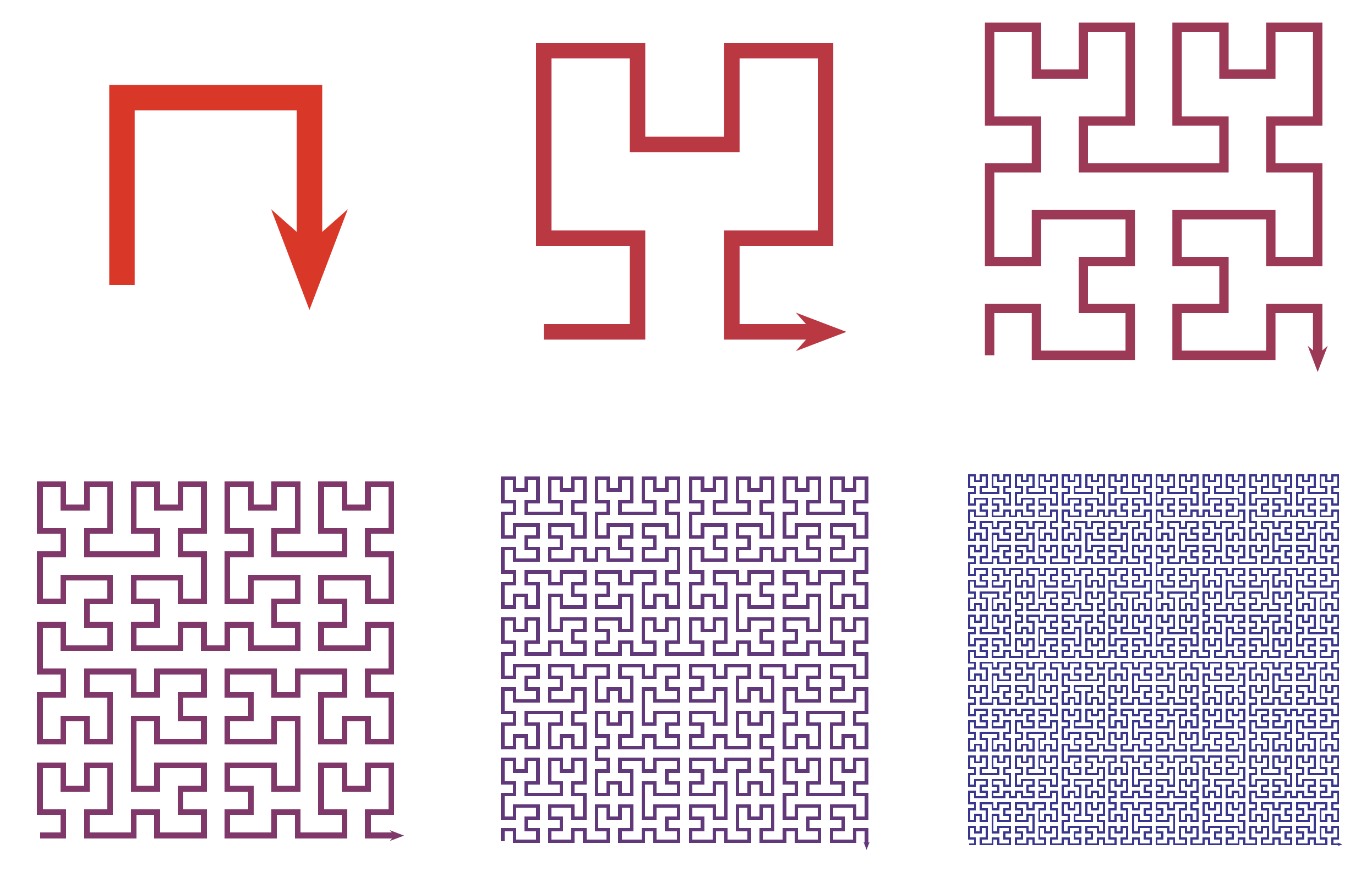
Each approximation curve traces a path in the plane—let us imagine them as describing the position of a figure skater performing an exhibition on ice in the town unit square. She enters the stage in each case at the lower left, makes an exhilarating performance with many twists and turns, and then exits at the lower right. With each successive performance, her skill increases, and she undertakes ever more intricate twists and turns. In the limit performance, her skating routine follows the fully space-filling figure-skating curve, visiting every point on the ice at some point during her performance. The limit path h(t) is a point describing her position at time t, which is the limit of the time-t positions as the approximations proceed.
One can begin to see this property already in the approximations to the Hilbert curve above. At the halfway point of each performance, the skater's path crosses from the left side of the ice to the right side—there is only one such crossing with each approximation—can you find it? These crossing points are converging to the very center of the square, and the halfway value h(½) of the limit path h will therefore be the point ( ½ , ½ ). Because the wriggling twists and turns are increasingly local, the limit curve will be continuous; and because the wriggling gets finer and finer and ultimately enters every region of the square, it follows that every point in the square will occur on the limit path. So the Hilbert curve is a space-filling curve. To my way of thinking, this example begins to stretch, or even break, our naive intuitions about what a curve is or what a function (or even a continuous function) can be.
Questions for further thought
What is your explanation for why it was generally the smaller country with the larger estimates for the length of a common border with another country?
Is the infinite coastline paradox about actual coastlines? Or is it instead only about the purely mathematical existence of curves and functions that behave differently from those in our ordinary experience?
Can you make a graph estimating the derivative of the elegant function from A to B considered in the chapter? What does it look like if the function is as well behaved as one might hope for? What does the derivative look like if the function has the small-scale monstrous nature discussed in the chapter?
Does the existence of nonrectifiable curves, including space-filling curves, challenge the coherence of the intuitive mathematical ideas we might have about the concept of the length of a curve?
Explain the meaning of Richardson's quotation, “Big whirls have little whirls that feed on their velocity; little whirls have lesser whirls & so on to viscosity.”
Furtherreading
The Wikipedia article on the coastline paradox is helpful.
Credits
Information about Lewis Fry Richardson was found in
Ryan Stoa, 2019. The coastline paradox. Rutgers University Law Review 72 (2): 351–400. doi:10.2139/ssrn.3445756. ssrn.com/abstract=3445756.
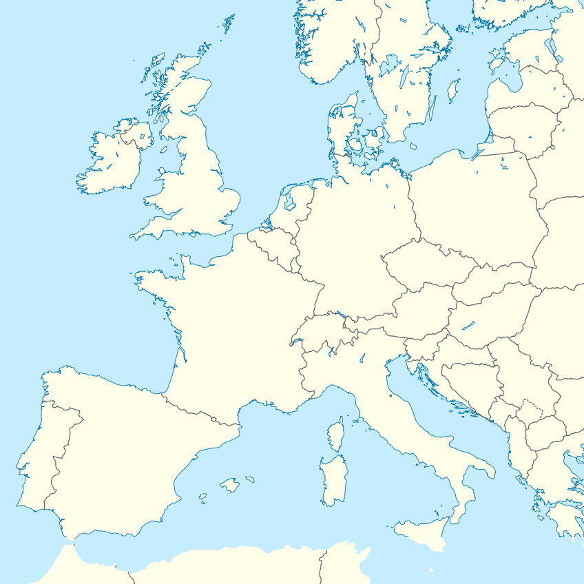
The map of Europe at the opening of the chapter was cropped from a map of user Alexrk2, CC BY-SA 3.0, via Wikimedia Commons. The animated map of the Great Britain coastline is due to user Tveness, CC0 via Wikimedia Commons. The figure on approximations of π is adapted from exercise 6.7 in my book:
Hamkins, Joel David. 2020. Proof and the Art of Mathematics. MIT Press. Available on Amazon.
and the related discussion in the supplement:
Hamkins, Joel David, 2021. Proof and the Art of Mathematics: examples and extensions. MIT Press. Available on Amazon.
The material on space-filling curves was adapted from section 2.6 in my book
Hamkins, Joel David, Lectures on the Philosophy of Mathematics. 2021. MIT Press. Available on Amazon.
"The final Hilbert curve itself is the limit of these approximations as they get finer and finer."
-----------------------------------------------------------------------------------------------------------------
If we create a computer program to iterate and output successive Hilbert curves, it will never output the final Hilbert curve since there is no last iteration. Does it exist? Is it fair to say that there is a final curve but not a final iteration? I think It might be reasonable to say that the final Hilbert curve is a 'mirage' (as opposed to an output) of the program. This may be a subtle distinction, but I think it's important because it puts the final Hilbert curve in a different class of existence than all the other Hilbert curves, one that doesn't rely on completing an infinite process. What do you think?
Thanks for the essay!!! I enjoyed reading it. In the space filling curve, it is claimed that the skater will visit "every point on the ice at some point during her performance”. I am wondering if this can give another characterisation of the dimension. For example, can I say that in Sierpinski gasket approximations, the skater will never visit certain points on the ice (which is the outer triangle), and the "proportion of these points on the ice" depends only on the dimension of the curve? (Is it measure theory that I need to study to be able to understand more about these results?)